 Linear regression is an old friend for me. I had made my first acquaintance with it already at the high school. It appeared and re-appeared again in several lectures at the University such as probability, signals and systems, statistics, digital filters and so on. I used it for both my semester and diploma thesis along with neural networks and genetic algorithms in the context of artificial intelligence. I used it even after the university in my professional life; for performance estimations in direct marketing, and for forecasts in financial planning to name some examples.
Its use is so widespread in quantitative models because linear regression is simple and effective. It is a good approximator and an excellent generalizer; it doesn’t suffer from the overtraining phenomenon sometimes observed with more complex predictive models like neural networks. I will come back to this training issue in this article.
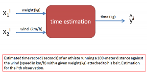
 This article is dedicated to the background theory. I will introduce here the mathematics of linear regression with a simple example. It is a predictive model for estimating the time record of an athlete (in seconds) running a 100-meter distance against the wind (speed in km/h) with a given weight (in kg) attached to his belt.
The cap symbol above “y” denotes estimation. Two independent input parameters weight (in kg) and wind (in km/h) are used as quantitative clues for estimating the time record. There are surely lots of other factors like weather temperature, time of the day and humidity affecting the performance of the athlete, but we have only two clues given for the estimation. All other unknown factors account for the uncertainty of the time estimation. That is why this is not a deterministic model; it delivers only an estimation.
 Assume that our athlete runs 300 times the same Strecke with different weights and wind conditions. In each run he records the weight, wind speed and time. These 300 measurements (observations) are our historical data.
 The time estimation y^ is calculated as a linear combination of the input parameters x1 and x2. This is actually what linear regression means. The output parameters like estimations or predictions are represented as linear combination of the input parameters. The rest of the problem is then optimizing the constant coefficients β so that the sum of squared deviations between the estimates and actual historical measurements are minimized (curve fitting).
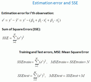
Normally, the historical data are divided into two parts. For example, randomly chosen 200 data sets of the 300 observations are used for training (training data). That is, for optimizing the β coefficients to minimize SSEtrain. Optimized β coefficients are then tested with the rest of the 100 observations (test data) to calculate SSEtest and MSEtest, and to check the precision and consistency of the predictive model. This test is done to check if the predictive model is ready for real estimations in future.
It is fine if MSEtrain is approximately equal to MSEtest. This means, the estimation model is general and consistent enough across different data sets. A significant deviation between MSEtrain and MSEtest is a bad sign, which might mean one or both of the followings:
- Due to the relatively high degree of freedom of model parameters (in our case β coefficients) compared to the number of observations in training data, the predictive model might have over-learned the training data (in a sense memorized rather than finding a general rule). The solution could be increasing the size of the training data; for example, 500 data sets instead of 200 for improved generalizations.
- For some reason, the test data might have a different statistical character than the training data. The reason can be a significant change in another implicit factor like temperature affecting the outcome. The temperature could be for example by chance much lower for the most of the training data compared to the test data.
 The historical data can be represented with matrices and vectors. This provides a more structured overview to the data. Furthermore, mathematical operations can easily be formulated with this matrix notation in an orderly manner.
The decisive question is, how can we calculate the optimal values of β coefficients that minimize the Sum of Square Error SSE? This will be handled in the following section.
Linear filters
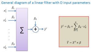
 Linear filter, a term often used in signal processing, is a more visual and intuitive way of displaying linear combination. The diagram above shows a generic linear filter with D input parameters. Each input parameter xj is weighted with its own coefficient βj. The estimated value y^ is the linear combination of all input parameters.
Optimal B coefficients that minimize SSE
 Assume that historical data (i.e. observations) are represented with the input matrix X and output vector Y. With this data we want to train and test the linear filter as our estimation model. Training means here adjusting the β coefficients so that the training error SSEtrain is minimized. This process can also be seen as curve fitting.
 With randomly chosen data sets we separate the historical data into two parts: Data sets for training and test. We have then training data Xtrain and Ytrain with N observations (i.e. data sets), test data Xtest and Ytest with M observations. N+M is the total number of data sets included in historical data.
Care should be taken so that:
- The number of observations (data sets) in training and test data should be sufficiently large to obtain statistically meaningful results. Small data sets can result in random rules or memorizing of the training data.
- The data sets for training and test data should be chosen randomly from the whole population of observations so that the training and test data represent similar data populations with comparable statistical characteristics.
 In order to find the formula for the optimal coefficient vector βopt we should formulate SSE as a function of β. By setting the derivative of this SSE function (derivative w.r.t. β) equal to zero, we can derive the formula for βopt that minimize SSE. This is exactly the same process where we want to find the x value that maximizes or minimizes f(x). We set the derivative df(x)/dx = 0, and solve it for x.
Calculate βopt with training data
 Now we have the general formula for the optimal β coefficients that minimize SSE. As already mentioned above, the optimal β coefficients should normally be calculated with the training data only. The mean square errors MSEtrain and MSEtest can then be calculated with these optimal coefficients. If MSEtrain is approximately equal to MSEtest, the predictive model with its tuned coefficients is ready for real estimations.
So much for the theory of linear regression. I plan to show the simple time estimation model introduced here in action in the following article. I will handle some interesting examples with linear regression models like weight guessing lottery or CDtoHome (direct marketing) in some other future articles. I will also tackle the quantifiable value of information in these examples for reducing uncertainty.
Tunç Ali Kütükçüoglu, 8. March 2012
Related content:
 Copyright secured by Digiprove © 2012 Tunc Ali Kütükcüoglu

