In this article, I will show the estimation model which was introduced in the previous related article in action with matlab and Simulink; estimating the time record of an athlete running 100-meters against the wind, with a weight attached to his belt. What can show something in action better than a video presentation? So let’s start with a short screencast.
The Pyhsical Function

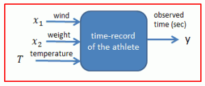
 I used this three-parameter function as shown on the left to generate historical data. The third factor temperature which is not captured by the estimation model represents generally all the unknown factors in the assumed physical reality (sounds like an oxymoron, isn’t it?) that add to the degree of uncertainty and estimation error in the time record of the athlete. In essence, the linear estimation model tries to approximate this three-parameter function with either one (cases 1 and 2) or two parameters (cases 3 and 4).
In the surface plot the left, you can see the observed time records of the athlete as a function of two factors, wind and temperature. The second factor weight is kept constant at 1 kg to generate this graph.
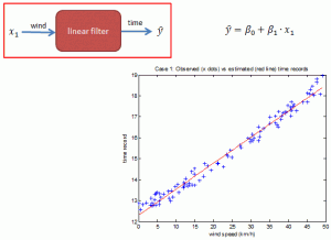
Case 1: Single-Parameter Time Estimation
 In this case, the estimation model tries to approximate the physical function which has three input factors with a single input factor only; wind speed. The estimation error is consequently quite high.
Case 2: Single-Parameter Polynomial Time Estimation
 The estimation error is slightly lower than that of the first case, because the quadratic component (i.e. square of wind speed) is also captured by this estimation model.
Case 3: Two-Parameter Time Estimation
 Here, the LR estimation model tries to guess the time-record of the athlete by capturing two of the three factors affecting the outcome; wind speed and weight. The expected estimation error is lower then the single-parameter case.
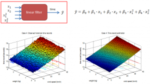
Case 4: Two-Parameter Polynomial Time Estimation
 Two factors, wind speed and weight are fully captured by this estimation model, including their quadratic components (i.e. square of). Accordingly, we can expect this model to have the lowest estimation error among the four.
A Comparison of Mean Square Errors (MSE)
 As expected, two-parameter estimations result in smaller estimation errors than the errors of the corresponding single-parameter models. Polynomial estimations result in smaller estimation errors because the physical function also includes the squares of the factors wind and weight.
What if we had a three-parameter polynomial estimation model with all the factors wind speed, weight and temperature, as input parameters? We would then have zero estimation error. But as mentioned before, the third factor temperature is not a single and simple input parameter; it symbolically represents all the unknown factors affecting the outcome, thereby adding to the uncertainty the estimation. Without this third factor, our case would not be an estimation model, as every estimation needs an element of uncertainty.
Tunç Ali Kütükçüoglu, 19. March 2012
You can download the supplementary PowerPoint slides and demonstration scripts for matlab and R from the download page. These demo scripts make all the calculations, and generate graphs for the four estimation cases mentioned in this article.
Related content:
 Copyright secured by Digiprove © 2012 Tunc Ali Kütükcüoglu

